Chapter 15 Tracing of Curves

15.1 Exercise 8

While tracing cartesian curves, look for mnemonic SONTRAD:

• Symmetry
• Origin
• Noticeable points
• Tangents
• Region
• Asymptotes
• Derivatives- first and second

To outline a general technique, we take these in turn.

• Where it crosses the -axis: The $x$-axis has equation $y=0$ and the curve has equation $y=f\left(x\right)$, so the curve crosses the $x$-axis at the points $(x,0)$ for which $f\left(x\right)=0$. Thus we solve the equation $f\left(x\right)=0$. This may have many solutions or none at all. (For instance, if $f\left(x\right)=\sin x$ there are infinitely many solutions, whereas if $f\left(x\right)=x^2+1$ there are none.)
• Where it crosses the $y$-axis: The $y$-axis has equation $x=0$ and the curve has equation $y=f\left(x\right)$ , so the curve crosses the $y$-axis at the single point $(0,f(0\left)\right)$.
• Finding the critical points: We have seen how to do this already. We solve the equation $f^{\prime }\left(x\right)=0$.
• The natures of the critical points: This means determining whether each one is a local maximum, local minimum, or inflexion point.
• Limiting behaviour: We have to determine what happens to $f\left(x\right)$ as $x$ tends to infinity and as $x$ tends to minus infinity; in other words, we have to ask how $f\left(x\right)$ behaves for $x$ far to the right on the $x$-axis and for $x$ far to the left on the negative side of the axis.

As far as the last point (limiting behaviour) is concerned, there are two standard results here which are useful.

First, the behaviour of a polynomial function is determined solely by its leading term, the one with the highest power of $x$. This term dominates for $x$ of large absolute value. A useful observation is that if $n$ is even, then

$$x^n\to \infty \text{as}x\to \infty \text{and also as}x\to -\infty$$

while if $n$ is odd,

$$f\left(x\right)\to \infty \text{as}x\to \infty \text{and}f\left(x\right)\to -\infty \text{as}x\to -\infty .$$

Secondly, whenever we have a function which is the product of an exponential and a power, the exponential dominates. Thus, for example, $x^2{\text{e}}^{-x}\to 0$ as $x\to \infty$ (even though $x^2\to \infty$).

15.1.1 Question 1

Trace the following curves

1. $y=(x^2-x-6)(x-7)$

• The equation can be written as $y=(x-3)(x+2)(x-7)$. So the curve passes through $(3,0),(-2,0),(7,0)$.
• Does not pass through origin.
• When $x=0$, $y=42$. The curve passes through $(0,42)$.
• $\frac{dy}{dx}=3x^2-16x+1$. So the tangents parallel to $x$-axis are at

$$\begin{array}{cc}\frac{dy}{dx}& =0\\ 3x^2-16x+1& =0\\ x& =5.27,0.06\end{array}$$

the coordinates $(5.27,28.55),(0.06,42.03)$

• $f^{\prime \prime }\left(x\right)=6x-16$. At $(5.27,28.55), $f^{\prime \prime }\left(x\right)$ is positive, so this is minima and at $(0.06,42.03)$, $f^{\prime \prime }\left(x\right)$ is negative, so this is maxima.
• The point of inflection

$$\begin{array}{cc}{f}^{\prime \prime }\left(x\right)& =0\\ 6x-16& =0\\ x& =2.67\end{array}$$

So at point $(2.67,6.67)$, the curve changes concavity from downward to upward.

• When $x\to \infty$, $y\to \infty$.

• When $x\to -\infty$, $y\to -\infty$.

With all these information, the curve can be easily plotted as below:

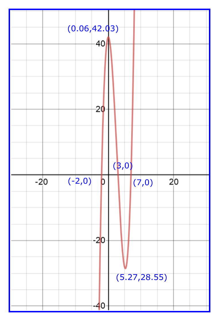
Figure 15.1: Tracing of $y=(x^2-x-6)(x-7)$

2. $\frac{2x-3}{x^2-3x+2}$

• The equation can be written as

$$\begin{array}{cc}y& =\frac{2x-3}{(x-1)(x-2)}\end{array}$$

• The curve is not symmetric around $x$ or $y$-axis.

• Does not pass through the origin.

• Vertical asymptotes are $x=1$ and $x=2$.

• When $x=0$, $y=-3/2$

• When $y=0$, $x=3/2$

• When $x\to +\infty$, $y\to +0$ and when $x\to -\infty$, $y\to -0$

• When $x\to 1^{-}$, $y\to -\infty$ and when $x\to 1^{+}$, $y\to +\infty$

• When $x\to 2^{-}$, $y\to -\infty$ and when $x\to 2^{+}$, $y\to +\infty$

• For maxima, minima

$$\begin{array}{cc}\frac{dy}{dx}& =\frac{2(x-1)(x-2)-(2x-3)(x-2)-(2x-3)(x-1)}{(x-1{)}^2(x-2{)}^2}\end{array}$$

Setting $\frac{dy}{dx}=0$

$$\begin{array}{cc}\frac{2(x-1)(x-2)-(2x-3)(x-2)-(2x-3)(x-1)}{(x-1{)}^2(x-2{)}^2}& =0\\ 2x^2-6x+5& =0\end{array}$$

$x$ is not defined, so the function does not have maxima or minima.

Thus the curve can be traced as shown below:

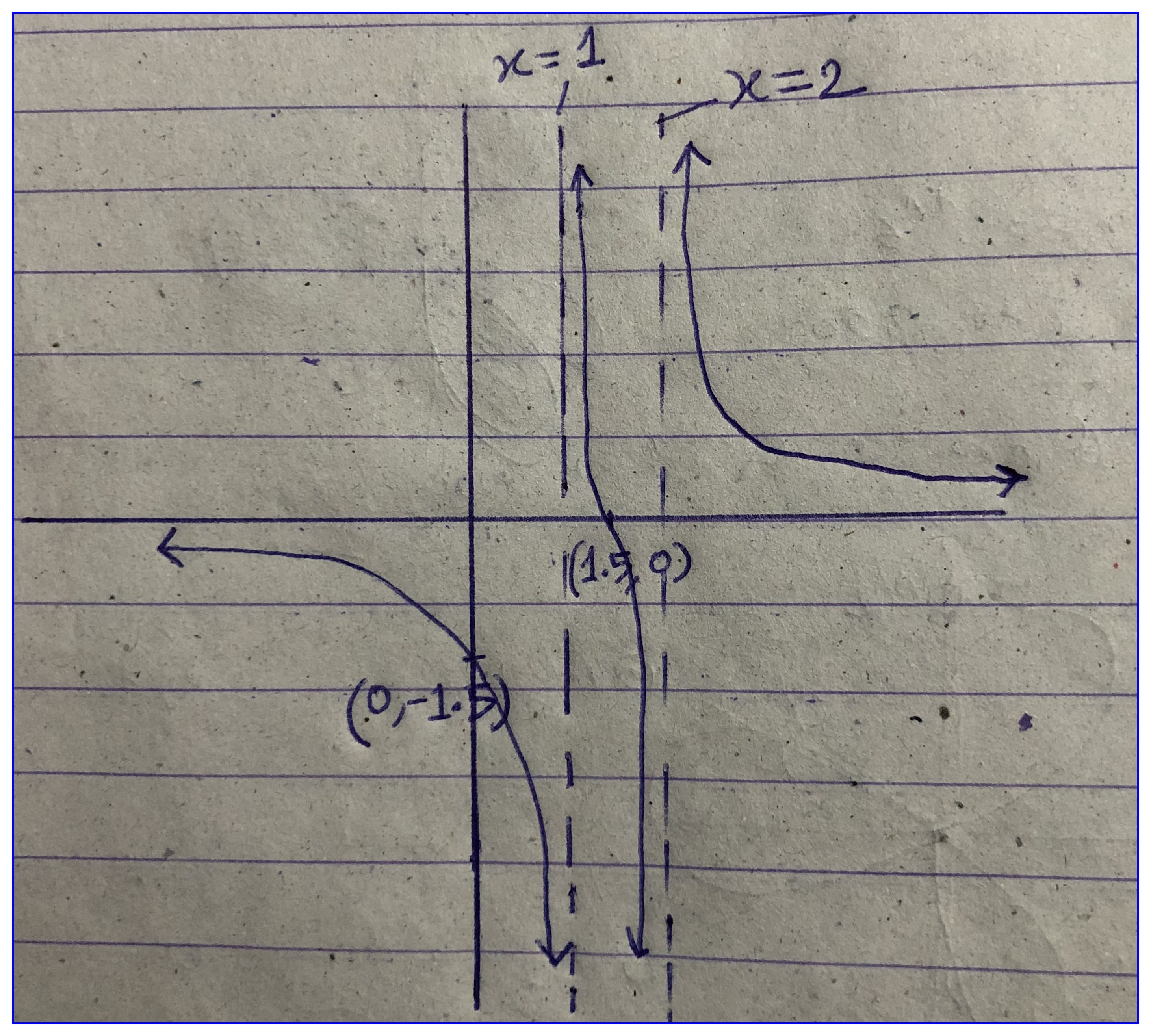
Figure 15.2: $y=\frac{2x-3}{x^2-3x+2}$

3. $y^2(a-x)=x^2(a+x)$

• The curve is symmetric about $x$-axis because the power of y is only even.

• Passes through origin.

• Tangents at origin are found by equating least powers of $x$ and $y$ to $0$

$$\begin{array}{cc}{y}^{2}a-x^{2}a& =0\\ y& =\pm x\end{array}$$

• When $y=0$, $x=0,-a$

• Domain: As the equation can also be written as $y=\sqrt{\frac{x^2(a+x)}{a-x}}$, the function won’t have real values if $x>a$ or $x<-a$. So the function is not defined in that region.

• The vertical asymptote is $x=a$.

• When $x\to a$, $y\to \pm \infty$

• $\frac{dy}{dx}$ is $\infty$ at $(-a,0)$. So the tangent is perpendicular at that point.

The curve is as shown below:

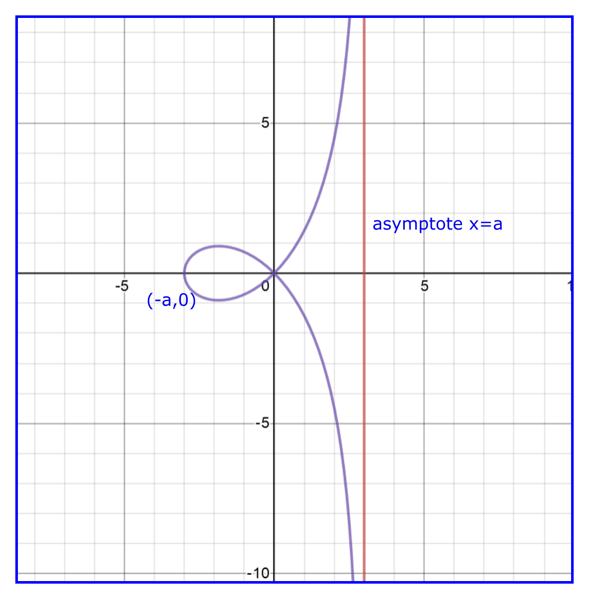
Figure 15.3: $y^2(a-x)=x^2(a+x)$

4. $x^2{y}^2=x^2-1$

• The curve is symmetric about both $x$ and $y$ axes as the power of $y$ and $x$ are only even.

• The equation can be written as $y^2=\frac{x^2-1}{x^2}$. The function is thus not defined between $(-1,1)$.

• When $x=-1,y=0$ and $x=1,y=0$

• When $x\to \infty$, $y=\pm 1$ and when $x\to -\infty$, $y=\pm 1$.

• Asymptotes parallel to $x$-axis

$$\begin{array}{cc}{y}^2-1& =0\\ y& =\pm 1\end{array}$$

• $\frac{dy}{dx}=\frac{1-y^2}{xy}$. Its value at $(-1,0)$ and at $(1,0)$ is $\infty$. So the tangents at these points are perpendicular at these points.

With this information, the curve can be easily traced as follows:

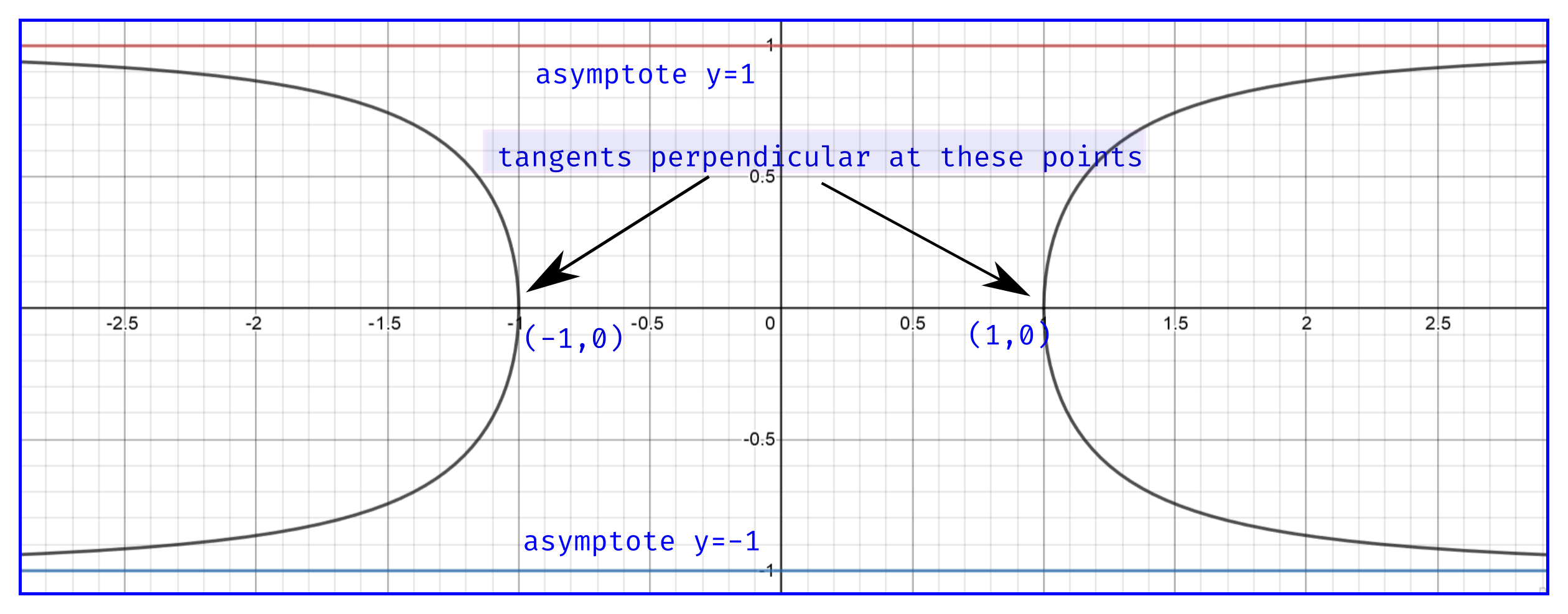
Figure 15.4: $x^2{y}^2=x^2-1$

22. $x^2(x^2+y^2)=a^2(x^2-y^2)$

• The curve is symmetric about both $x$ and $y$-axes as powers of $y$ and $x$ are only even.

• Passes through origin.

• Tangents at origin

$$\begin{array}{cc}{x}^2{a}^2& =y^2{a}^2\\ y& =\pm x\end{array}$$

• No asymptotes parallel to $x$ or $y$ axis.

• When $y=0$, $x=\pm a$. Passes through $(a,0)$ and $(-a,0)$.

• The equation can be written as $y^2=\frac{x^2{a}^2-x^4}{x^2+a^2}$. Thus curve is not defined when $x>a$ or $x<-a$.

• To find the slope of tangents at $(a,0)$ and $(-a,0)$, let us find $\frac{dy}{dx}$

$$\begin{array}{cc}\frac{dy}{dx}& =\frac{a^{2}x-2x^3}{x^{2}y+a^{2}y}\end{array}$$

Slope of tangents at $(a,0)$ and $(-a,0)$ is $\infty$. Thus tangents are perpendicular at these points.

The curve is plotted as shown below:

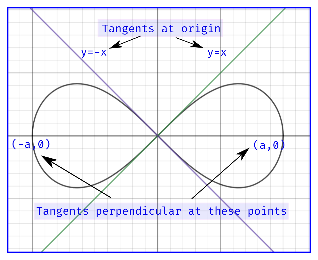
Figure 15.5: $x^2(x^2+y^2)=a^2(x^2-y^2)$

6. $y^2=x^3(4-x)$

• The curve is symmetric around $x$-axis as the power of y is only even i.e equal to $2$.

• Passes through origin.

• No asymptotes parallel to $x$ or $y$ axis.

• When $y=0$, $x=0$ and $x=4$. The curve thus passes through $(0,0)$ and $(4,0)$.

• The curve is not defined at $x<0$ and $x>4$.

• $\frac{dy}{dx}$

$$\begin{array}{cc}2y\frac{dy}{dx}& =12x^2-4x^3\\ \frac{dy}{dx}& =\frac{6x-2x^2}{\sqrt{x(4-x)}}\end{array}$$

The tangents to the curve are parallel to the $x$-axis at $\frac{dy}{dx}=0$

$$\begin{array}{cc}\frac{6x-2x^2}{\sqrt{x(4-x)}}& =0\\ 2x^2-6x& =0\\ x(x-3)& =0\\ x& =0,3\end{array}$$

So at $(0,0),(3,5.2)$ and $(3,-5.2)$ tangents are parallel to $x$-axis.

• At $(4,0)$, $\frac{dy}{dx}=\infty$. So tangent is perpendicular at this point.

• = . At $(3,5.2)$, $f^{\prime \prime }\left(x\right)$ is negative, therefore it is maxima and at $(3,-5.2)$, $f^{\prime \prime }\left(x\right)$ is positive, therefore it is minima.

• Point of inflection is where $f^{\prime \prime }\left(x\right)=0$

$$\begin{array}{cc}{f}^{\prime \prime }\left(x\right)& =0\\ 6x^2-12x& =0\\ x(x-2)& =0\\ x& =0,2\end{array}$$

So $(0,0)$ and $(2,4)$ are points of inflection where curve changes concavity.

Thus we completed the upper half of this curve. As it is symmetric to $x$-axis, the lower half can be plotted as a reflection of upper half.

Thus curve is easily plotted as shown below:

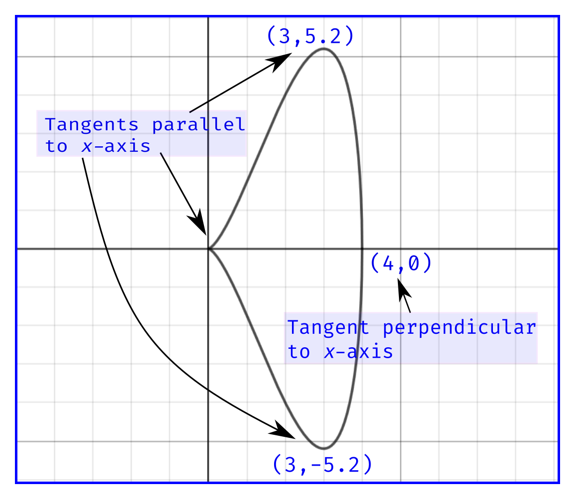
Figure 15.6: $y^2=x^3(4-x)$

Few famous curves:

• Folium of Descartes
• Cissoid of Diocles
• Witch of Agnesi
• Strophoid

15.1.2 Question 2

Trace the following curves

1. $a^2{b}^2+x^2{y}^2=a^2{x}^2$

• The curve is symmetric about both $x$ and $y$ axes.

• Does not pass through origin.

• The equation can be written as $y^2=\frac{a^2{x}^2-a^2{b}^2}{x^2}$. The curve is thus not defined in the interval $(-b,b)$. It is defined only for $x\ge b$ and $x\le -b$.

• When $y=0$, $x=\pm b$. The curve thus passes through $(b,0)$ and $(-b,0)$.

• Asymptotes parallel to $x$-axis are $y=\pm a$.

• $\frac{dy}{dx}=\frac{a^2-y^2}{xy}$. So at point $(b,0)$ and $(-b,0)$, slope is $\infty$, so tangents are perpendicular at these two points.

The curve is thus plotted as:

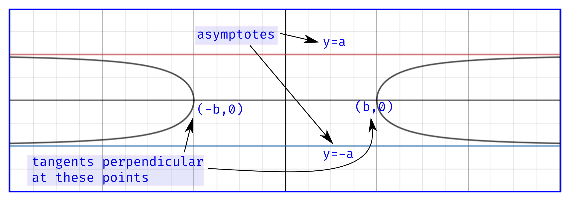
Figure 15.7: $a^2{b}^2+x^2{y}^2=a^2{x}^2$

2. $x^2(a^2+y^2)=y(a^2-y^2)$

• The curve is symmetric around $y$-axis.

• When $x=0$, $y=0,\pm a$. The curve passses through points $(0,0)$ (origin), $(0,a)$ and $(0,-a)$.

• No asymptotes parallel to $x$-axis.

• No asymptotes parallel to $y$-axis.

• Domain: $x^2=\frac{y(a^2-y^2)}{a^2+y^2}$. So when $y>a$ or $y$ lies in the interval $(0,-a)$, the curve is not defined.

• $\frac{dy}{dx}=\frac{2a^{2}x+2x{y}^2}{a^2-3y^2-2x^{2}y}$. At the points $(0,0)$ (origin), $(0,a)$ and $(0,-a)$, the tangents are parallel to $x$-axis.

• When $y\to -\infty$, $x\to \pm \infty$.

The curve is thus plotted as below:

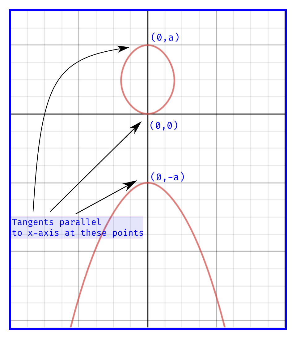
Figure 15.8: $x^2(a^2+y^2)=y(a^2-y^2)$

3. $y^2=x^2(a^2-x^2)$

• Symmetric around both $x$ and $y$ axes.

• Passes through the origin.

• When $y=0$, $x=0,\pm a$. So the curve passes through $(0,0)$, $(a,0)$ and $(-a,0)$.

• The function not defined when $x>a$ and $x<-a$.

• No asymptotes parallel to $x$ or $y$ axis.

• Slope

$$\begin{array}{cc}\frac{dy}{dx}& =\frac{a^{2}x-2x^3}{y}\\ & =\pm \frac{a^2-2x^2}{\sqrt{a^2-x^2}}\end{array}$$

• Slope at origin $(0,0)$ is $\pm a$.

• Slope at $(a,0)$ and $(-a,0)$ is $\infty$. So tangents to the curve at these points are perpendicular to $x$-axis.

• $\frac{dy}{dx}=0$ is at $x=\pm \frac{a}{\sqrt{2}}$. The tangents are parallel to $x$-axis at $x=\pm \frac{a}{\sqrt{2}}$ and $y=\pm \frac{a^2}{2}$.

• Point of inflection

$$\begin{array}{cc}\frac{d^{2}y}{d{x}^2}& =\frac{a^2-6x^2}{y+1}\end{array}$$

$$\begin{array}{cc}\frac{d^{2}y}{d{x}^2}& =0\\ \frac{a^2-6x^2}{y+1}& =0\\ x& =\pm \frac{a}{\sqrt{6}}\end{array}$$

The point of inflection is $(\pm \frac{a}{\sqrt{6}},\pm \frac{\sqrt{5}{a}^2}{6})$.

With this information curve is easily plotted as follows:

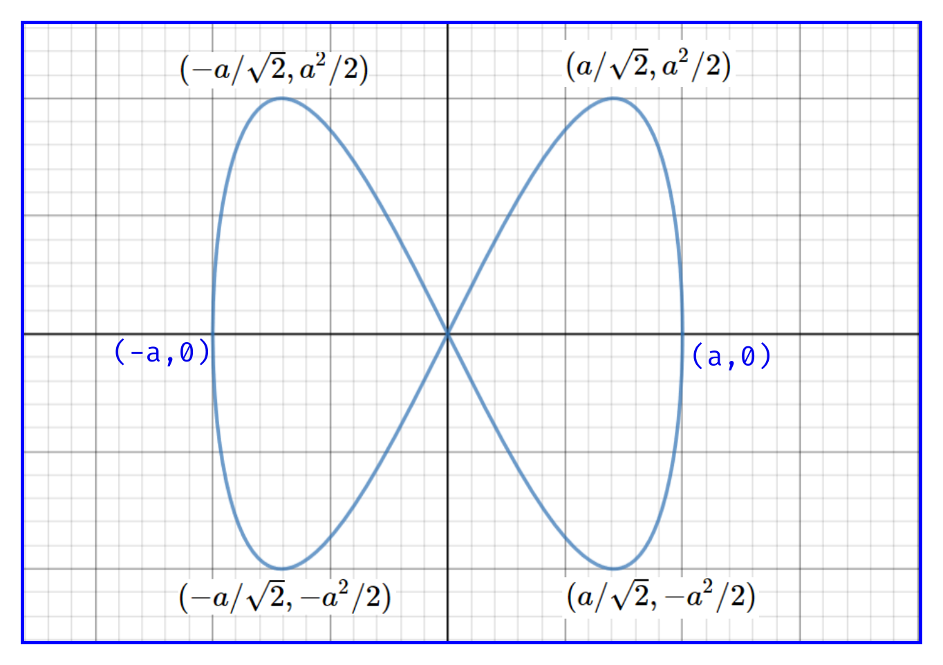
Figure 15.9: $y^2=x^2(a^2-x^2$

4. $y^2=x^3$

• The curve is symmetric about $x$-axis.

• Domain: $[0,\infty )$

• Passes through origin.

• When $x\to \infty$, $y\to \pm \infty$.

• $\frac{dy}{dx}=\pm \frac{3}{2}\sqrt{x}$. $\frac{dy}{dx}=0$ at $x=0$ i.e at origin.

• So as $x$ increases slope also increases.

• No asymptotes parallel to $x$ or $y$ axis.

• $\frac{d^{2}y}{d{x}^2}=\frac{3x}{y+1}$. The point of inflection is at $x=0$.

The graph is easily plotted as:

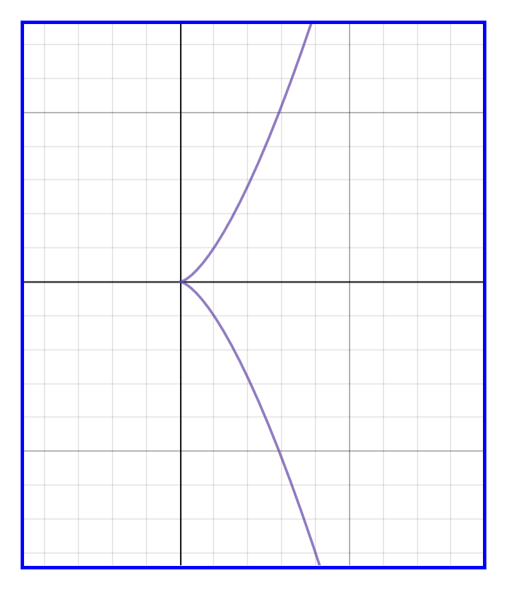
Figure 15.10: $y^2=x^3$

22. $y^2=(x-2a{)}^3$

• The curve is symmetric about $x$-axis.

• Does not pass through origin.

• When $y=0$, $x=2a$. Passes through $(2a,0)$.

• Domain: $[2a,\infty )$. Function not defined when $x<2a$.

• $\frac{dy}{dx}=\pm \frac{3}{2}\sqrt{x-2a}$. It is $0$ when $x=2a$.

• Beyond $x=2a$, slope continuously increases.

• Point of inflection is $x=2a$.

• No asymptotes parallel to $x$ or $y$ axis.

The curve is as shown below:

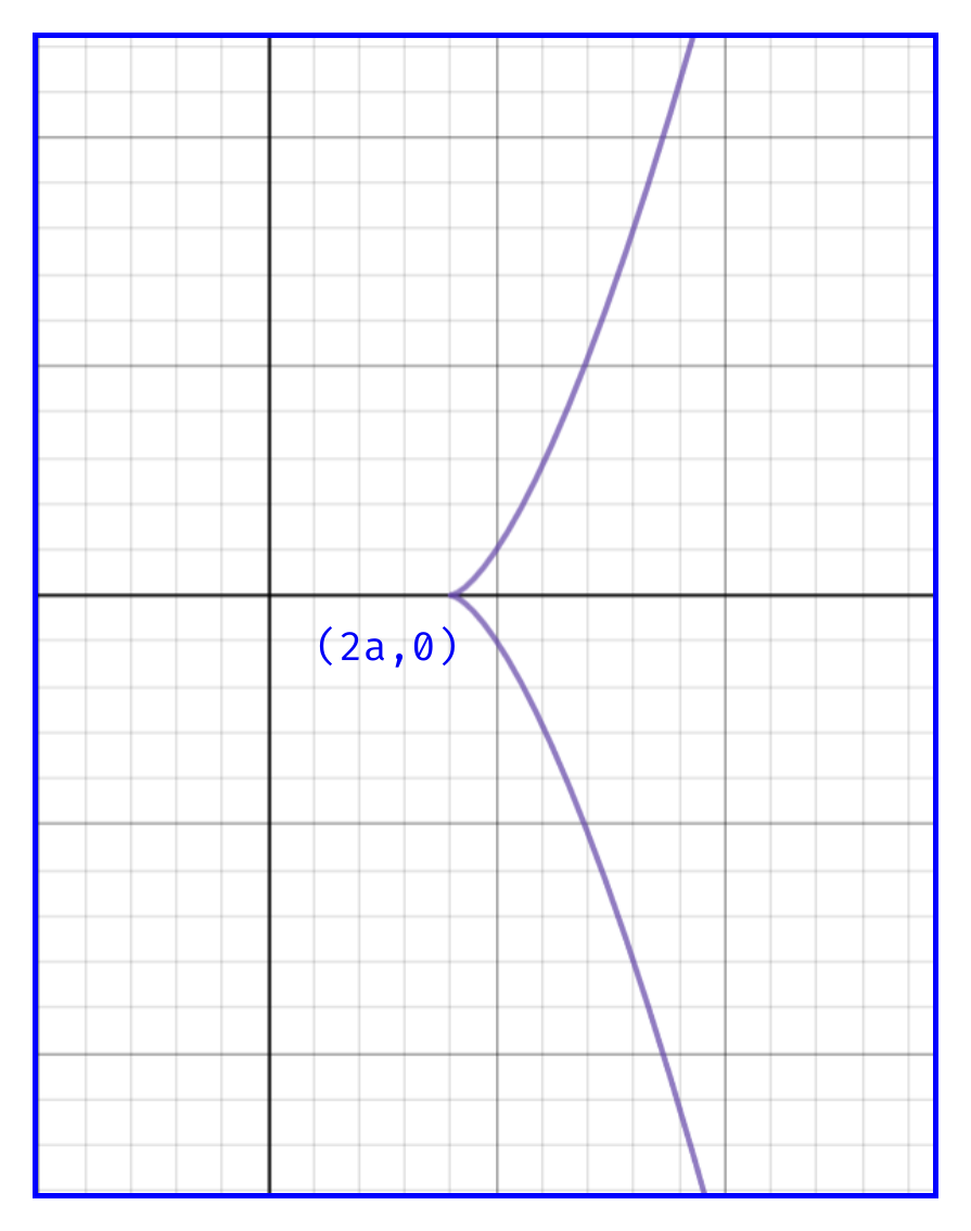
Figure 15.11: $y^2=(x-2a{)}^3$

6. $x^2{y}^2=a^2(y^2-x^2)$

• The curve is symmetric about both $x$ and $y$ axes.

• Passes through origin.

• No asymptotes parallel to $x$-axis.

• Asymptotes parallel to $y$-axis are $x=\pm a$.

• Domain of the given function $y^2=\frac{a^2{x}^2}{a^2-x^2}$ is $(-a,a)$. It is not defined when $x\ge a$ or $x\le -a$.

• When $x\to a^{-}$, $y\to \pm \infty$.

• When $x\to -a^{+}$, $y\to \pm \infty$.

The curve is as shown below:

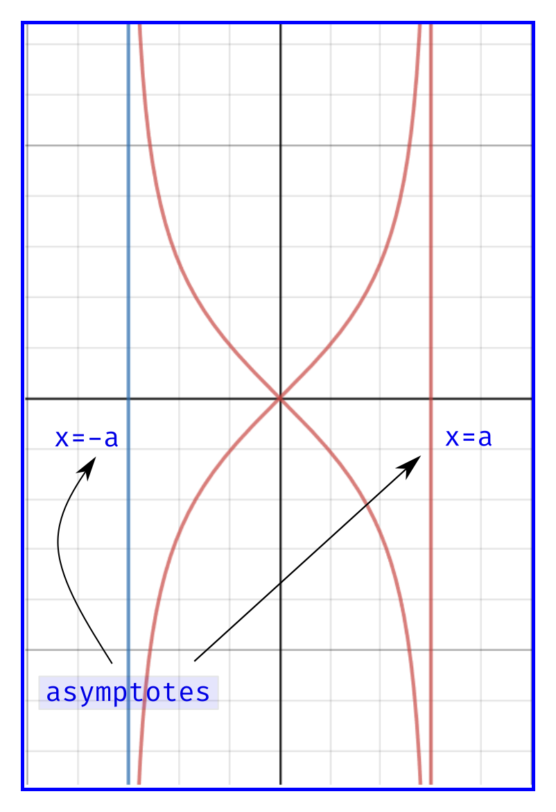
Figure 15.12: $x^2{y}^2=a^2(y^2-x^2)$

7. $y^2=x^2(a-x)$

• The curve is symmetric around $x$-axis.

• Passes through origin.

• When $y=0$, $x=0,a$. The curve thus passes through $(0,0)$, $(a,0)$.

• Domain: $(-\infty ,a]$.

• $\frac{dy}{dx}$

$$\begin{array}{cc}\frac{dy}{dx}& =\pm \frac{2a-3x}{2\sqrt{a-x}}\end{array}$$

$\frac{dy}{dx}=0$ when $x=\frac{2a}{3}$. When $x=\frac{2a}{3}$, $y=\pm \sqrt{\frac{4a^3}{27}}$. Thus tangents are parallel to $x$-axis at points $(x=\frac{2a}{3},\sqrt{\frac{4a^3}{27}})$ and $(x=\frac{2a}{3},-\sqrt{\frac{4a^3}{27}})$.

• Point of inflection is where $f^{\prime \prime }\left(x\right)=0$. In this case it is at $x=\frac{a}{3}$.

• $\frac{dy}{dx}$ at origin is $\pm \sqrt{a}$.

• $\frac{dy}{dx}$ at $(a,0)$ is $\infty$. Tangent is thus perpendicular here.

The curve thus can be very easily plotted as shown below:

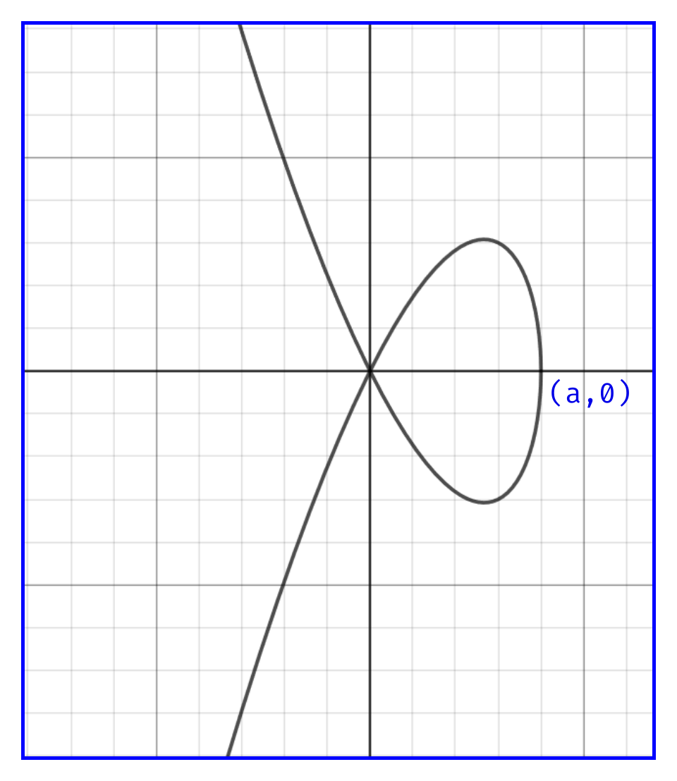
Figure 15.13: $y^2=x^2(a-x)$

15.1.3 Question 3

Trace the following curves

1. $r=a(1-\cos \theta )$

• $\cos \theta$ can range from $-1$ to $1$. So $r$ cannot be more $2a$.
• Replacing $\theta$ with $-\theta$ does not change the equation, so the curve is symmetric about the initial line i.e $\theta =0$ line.
• Values of $r$ at different $\theta$ values

$\theta$	$r$
$0$	$0$
$\pi /4$	$a(1-1/\sqrt{2})\approx 0.29a$
$\pi /3$	$a/2=0.5a$
$\pi /2$	$a$
$\pi$	$2a$
$2\pi$	$0$

• To find the tangents, we have to find $\tan \varphi =r\frac{d\theta }{dr}$

$$\begin{array}{cc}\tan \varphi & =r\frac{d\theta }{dr}\\ & =\tan \frac{\theta }{2}\\ \varphi & =\frac{\theta }{2}\end{array}$$

And

$$\begin{array}{cc}\psi & =\varphi +\theta \\ \psi & =\frac{\theta }{2}+\theta \\ & =\frac{3\theta }{2}\end{array}$$

The angle that tangents make at $\theta$ are:

$\theta$	$\psi$
$0$	$0$
$\pi$	$3\pi /2$

• Value of $r$ progressively increases from $\theta =0$ to $\theta =\pi$.
• As the curve is symmetric about initial line, the curve can be plotted as below:

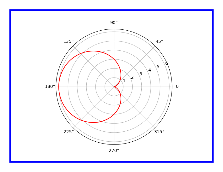
Figure 15.14: Plotting of $r=a(1-\cos \theta )$

2. $r^2=a^2\sin 2\theta$

• On replacing $r$ by $-r$, the equation does not change, so the curve is symmetrical about pole (called as origin in cartesian system).
• $r^2$ is negative when $\sin 2\theta$ is negative i.e when $\theta$ lies in open interval $(\pi ,2\pi )$ and $(\frac{3\pi }{2},2\pi )$. Thus the curve has no portion in these region.
• We know

$$\begin{array}{cc}\tan \varphi & =r\frac{d\theta }{dr}\\ \tan \varphi & =\frac{r^2}{a^2\cos 2\theta }\\ \tan \varphi & =\tan 2\theta \\ \varphi & =2\theta \end{array}$$

and

$$\begin{array}{cc}\psi & =\varphi +\theta \\ \psi & =2\theta +\theta \\ \psi & =3\theta \end{array}$$

$\theta$	$\psi$
$0$	$0$
$\pi /2$	$3\pi /2$
$\pi$	$3\pi$
$3\pi /2$	$9\pi /2$

• $r$ increases when $\theta$ increases from $0$ to $\pi /4$. $r$ will have two values for each $\theta$ in the region where curve is defined.

With these information curve is plotted as shown below:

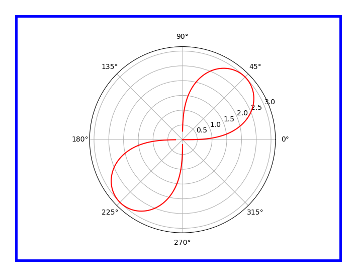
Figure 15.15: Plotting of $r^2=a^2\sin 2\theta$

• To trace curves of the form $r=a\sin n\theta$ or $r=a\cos n\theta$, know that since $\sin n\theta$ or $\cos n\theta$ cannot be greater than one in both the cases $r$ cannot be greater than $a$. Hence, the curve wholly lies within the circle of radius $a$.
• To find the curve $r=a\sin n\theta$ put $r=0$. Then $n\theta =0,\pi ,2\pi ,\cdots$ $$\theta =0,\frac{\pi }{n},\frac{2\pi }{n},\cdots$$ Draw these lines. If $n$ is odd there are $n$ loops in alternate divisions and if $n$ is even there are $2n$ loops one in each division.
• To trace the curve $r=a\cos n\theta$ put $r=0$ Then, $$\begin{array}{cc}n\theta & =-\frac{\pi }{2},\frac{\pi }{2},\frac{3\pi }{2},\frac{5\pi }{2},\cdots \\ \theta & =-\frac{\pi }{2n},\frac{\pi }{2n},\frac{3\pi }{2n},\frac{5\pi }{2n},\cdots \end{array}$$

Draw these lines. If $n$ is odd there are $n$ loops in alternate divisions and if $n$ is even there are $2n$ loops one in each division.

3. $r=a\cos 2\theta$

• Since $\cos 2\theta$ cannot be greater than $1$ (as cosine values range from $-1$ to $1$), $r$ cannot be greater than $a$.
• Replacing $\theta$ with $-\theta$ does not change the equation, so the curve is symmetric about the initial line.
• It is of form $r=a\cos n\theta$, with $n$ being even so the equation has $4$ loops.
• Putting $r=0$, then

$$\begin{array}{cc}\cos 2\theta & =0\\ 2\theta & =\frac{\pi }{2},\frac{3\pi }{2},\frac{5\pi }{2},\frac{7\pi }{2},\cdots \\ \theta & =\frac{\pi }{4},\frac{3\pi }{4},\frac{5\pi }{4},\frac{7\pi }{4},\cdots \end{array}$$

Draw these lines, and as $2$ is even there are total $4$ loops one in each division.

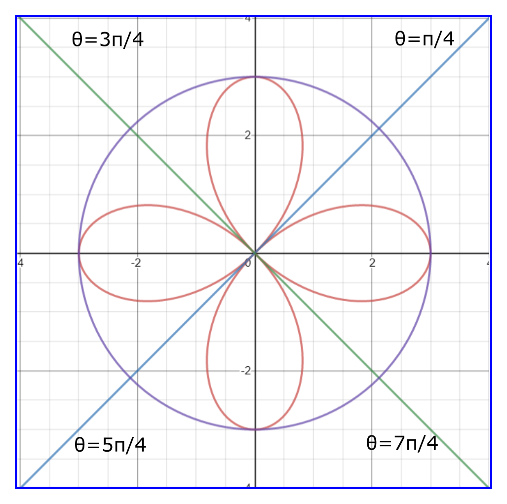
Figure 15.16: Plotting of $r=a\cos 2\theta$

4. $r=a\cos 3\theta$

• Since $\cos 3\theta$ cannot be greater than $1$, $r$ cannot be greater than $a$.
• Replacing $\theta$ with $-\theta$ does not change the equation, so the curve is symmetric about the initial line.
• It is of form $r=a\cos n\theta$, so the equation has $3$ loops.
• Putting $r=0$, then

$$\begin{array}{cc}\cos 3\theta & =0\\ 3\theta & =\frac{\pi }{2},\frac{3\pi }{2},\frac{5\pi }{2},\frac{7\pi }{2},\cdots \\ \theta & =\frac{\pi }{6},\frac{3\pi }{6},\frac{5\pi }{6},\frac{7\pi }{6},\cdots \end{array}$$

Draw these lines, and as $3$ is odd there are $3$ loops in alternate divisions.

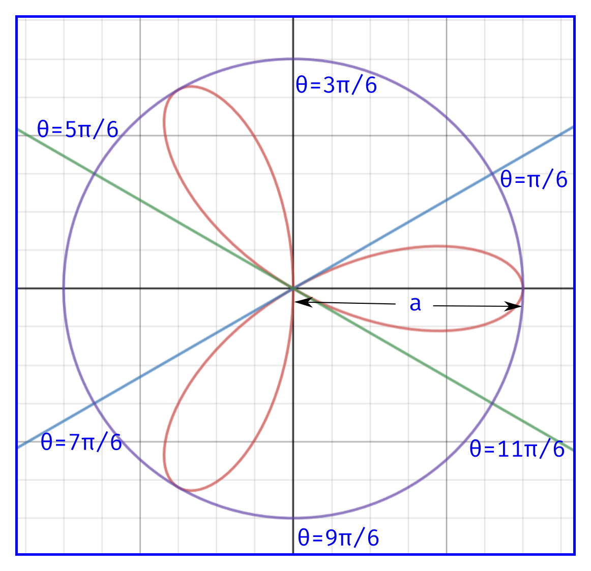
Figure 15.17: Plotting of $r=a\cos 3\theta$

15.1.4 Additional interesting questions

Trace the following curves

1. $y^2(x-a)=x^2(x+a)$

Please note $y^2(a-x)=x^2(x+a)$ gives a totally different curve. Try yourself !

• The curve is symmetric around $x$-axis as power of $y$ is even.
• When $y=0$, $x=0,x=-a$
• Domain: $y^2=\frac{x^2(x+a)}{x-a}$, the curve is not defined in the interval $(0,a),(-a,0)$.
• Asymptotes parallel to $y$-axis is obtained by equating coefficients of $y^2$, $$x=a$$
• The oblique asymptotes are (see chapter 13 for tricks: method of substitution of $x=1$, $y=m$) are $y=x+a$ and $y+x+a=0$.
• $\frac{dy}{dx}$

$$\begin{array}{cc}y& =\frac{x(x+a{)}^{1/2}}{(x-a{)}^{1/2}}\\ \frac{dy}{dx}& =\frac{(x-a{)}^{1/2}[\frac{x}{2(x+a{)}^{1/2}}+(x+a{)}^{1/2}]-x(x+a{)}^{1/2}\times \frac{1}{2(x-a{)}^{1/2}}}{x-a}\\ \frac{dy}{dx}& =\frac{(x-a{)}^{1/2}\left[\frac{x+2(x+a)}{2(x+a{)}^{1/2}}\right]-\frac{x(x+a{)}^{1/2}}{2(x-a{)}^{1/2}}}{x-a}\end{array}$$ Tangents to the curve is at where $dy/dx=0$, so

$$\begin{array}{cc}(x-a{)}^{1/2}\left[\frac{x+2(x+a)}{2(x+a{)}^{1/2}}\right]-\frac{x(x+a{)}^{1/2}}{2(x-a{)}^{1/2}}& =0\\ (x-a{)}^{1/2}\left[\frac{x+2(x+a)}{2(x+a{)}^{1/2}}\right]& =\frac{x(x+a{)}^{1/2}}{2(x-a{)}^{1/2}}\\ 2(x-a)(3x+2a)& =2x(x+a)\\ 3x^2+2ax-3ax-2a^2& =x^2+ax\\ x^2-ax-a^2& =0\end{array}$$ So the value of $x$, where slope is $0$ are:

$$\begin{array}{cc}x& =\frac{a\pm \sqrt{a^2+4a^2}}{2}\\ & =a\left(\frac{1\pm \sqrt{5}}{2}\right)\\ x& =1.61a,-0.62a\end{array}$$

Of the two $x$-values, $-0.62a$ does not lie within the domain of the given function, so we reject it.

• As $x>1.61a$, the value of numerator in $y^2=\frac{x^2(x+a)}{x-a}$ increases faster than the denominator. Hence value of $y$ increases more for even a small increase in $x$. Thus slope increases as $x$ increases beyond $x>1.61a$.

• At $x=1.61a$, $y=\pm 3.33a$.

• We know

$$\begin{array}{cc}2y\frac{dy}{dx}& =\frac{(x-a)[x^2+(x+a\left)2x\right]+x^2(x+a)}{(x-a{)}^2}\end{array}$$

so at point $(-a,0)$, $\frac{dy}{dx}=\infty$ i.e. tangent is perpendicular at this point.

• As $x$ decreases from $-a$ to $-\infty$, the value of $y$ also increases rapidly. And we know the curve is symmetric about $x$-axis.

With all these information the curve is easily plotted below:

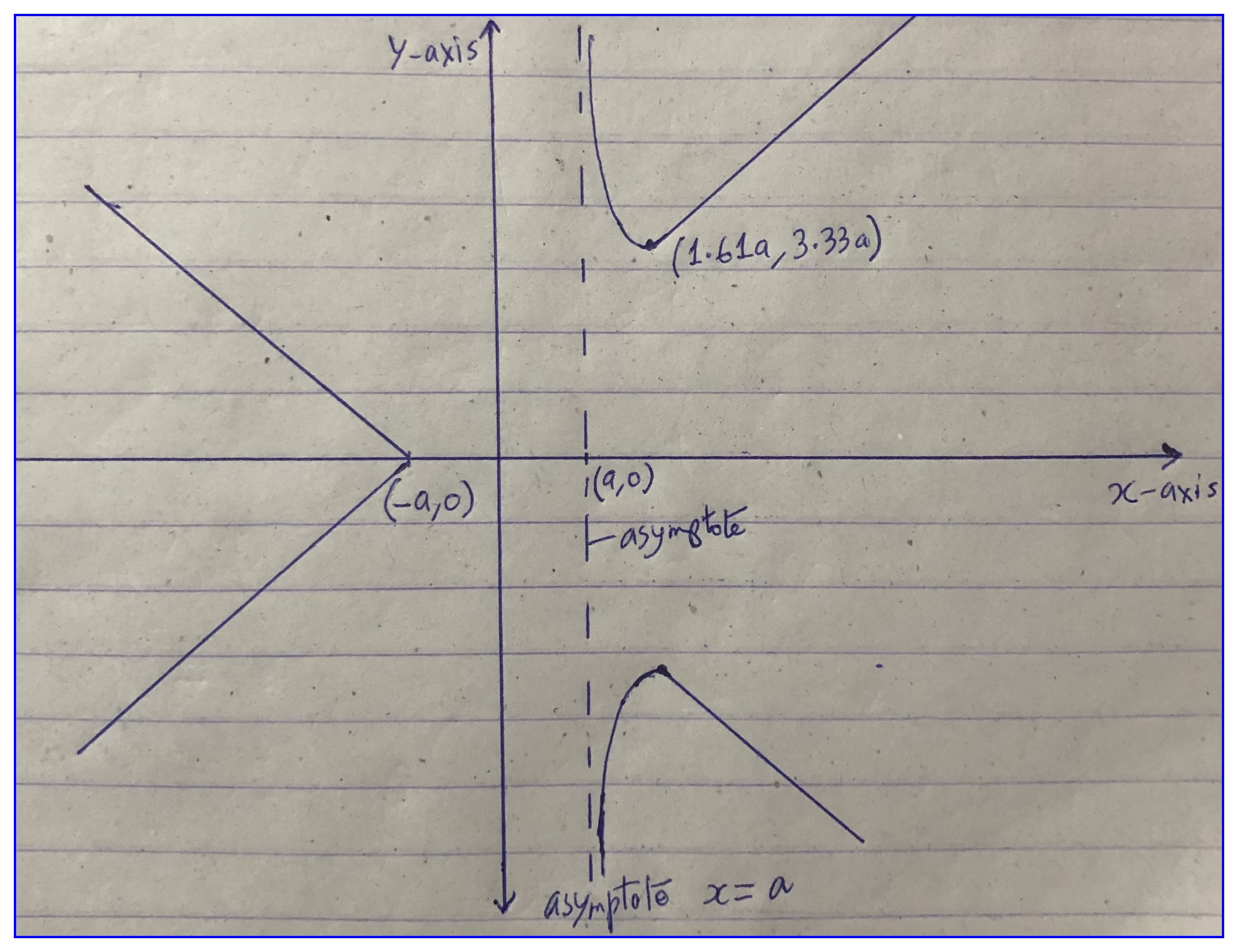
Figure 15.18: Curve for $y^2(x-a)=x^2(x+a)$

2. $y^2(x^2-4)=x^4$

• The curve is symmetric around both $x$ and $y$-axes.
• As $y^2=\frac{x^4}{x^2-4}$, the domain of the given function is $(-\infty ,2)$ and $(2,\infty )$. The function is not defined in the interval $[-2,2]$ except at the origin.

$$\begin{array}{}\begin{array}{cc}{y}^2& =\frac{x^4}{x^2-4}\end{array}& \text{(15.1)}\end{array}$$

• The asymptotes parallel to $y$-axis are $x=\pm 2$.
• No horizontal asymptotes
• The oblique asymptotes are $y=x$ and $y=-x$.
• Working for $\frac{dy}{dx}$

$$\begin{array}{cc}y& =\frac{x^2}{(x^2-4{)}^{1/2}}\\ \frac{dy}{dx}& =\frac{(x^2-4{)}^{1/2}\times 2x-x^2\times \frac{2x}{2(x^2-4{)}^{1/2}}}{x^2-4}\\ & =\frac{4x(x^2-4)-2x^3}{2(x^2-4{)}^{3/2}}\end{array}$$

To find maxima or minima,

$$\begin{array}{cc}\frac{dy}{dx}& =0\\ \frac{4x(x^2-4)-2x^3}{2(x^2-4{)}^{3/2}}& =0\\ 4x(x^2-4)& =2x^3\\ x& =\pm \sqrt{8}\end{array}$$

When $x=+\sqrt{8}$, $y=\pm 4$. When $x=-\sqrt{8}$, $y=\pm 4$.

• When $x\to 2^{+}$, $y\to \pm \infty$.

• When $x\to -2^{-}$, $y\to \pm \infty$.

• As value of $x>2$ to $+\infty$ or $x<-2$ to $-\infty$ in equation (15.1) value of numerator increases rapidly than denominator i.e. for even small increase in $x$, increase in $y$ is higher, so slope increases as $x\to \infty$ from $>2$. Hence curve will be concave upward. By symmetry the curve can be constructed as follow:

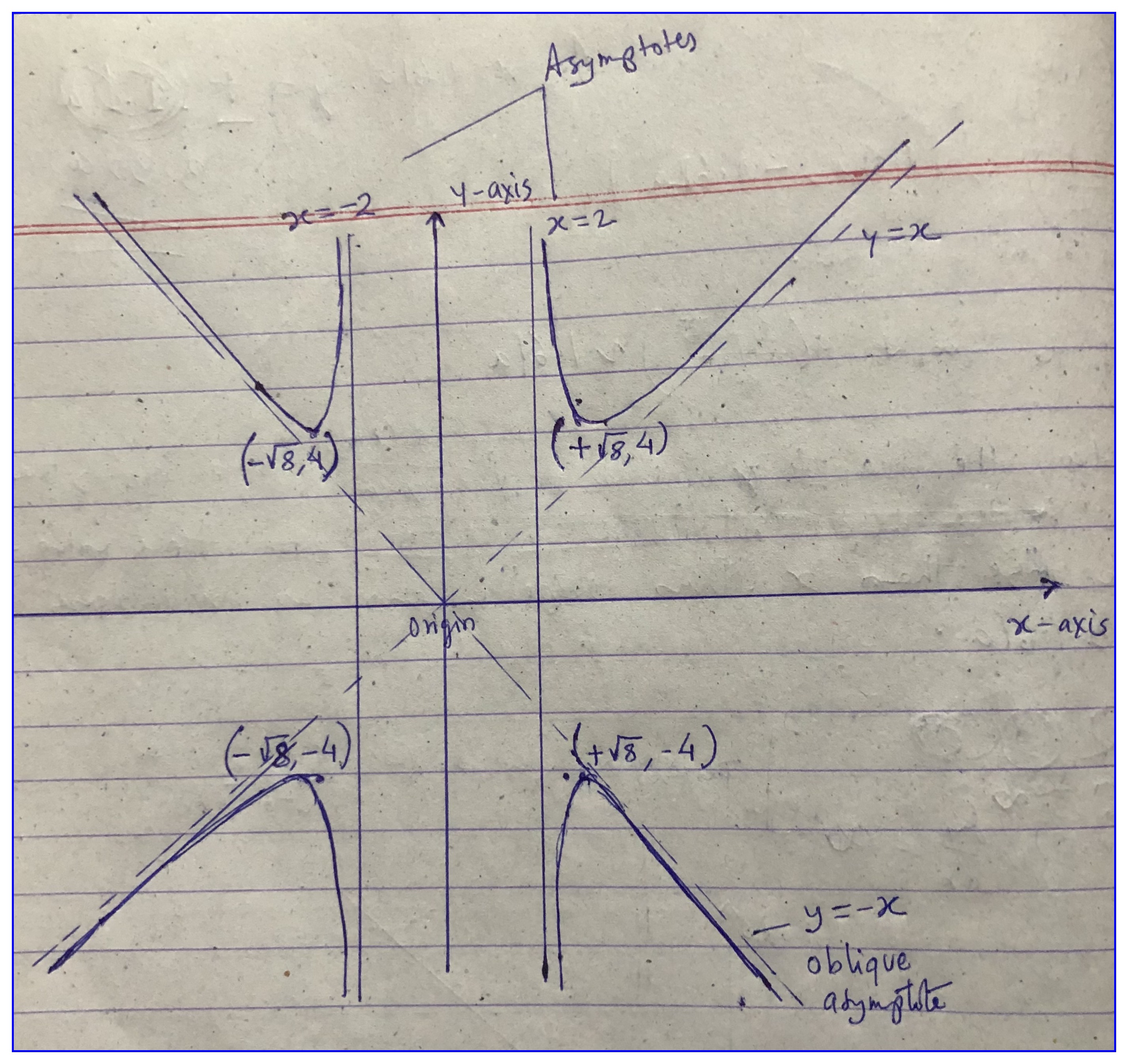
Figure 15.19: Curve of equation $y^2(x^2-4)=x^4$

Reading this on math stackexchange is useful. It explains the essential concepts.

15.2 Additional problems

1. $y=\sqrt{x^6+5}-x^3$

2. $y=\sqrt{x^6+5x^3}-x^3,x\ge 0$

3. $x^4+y^4=16$

4. $y^3+x^{2}y+x^2-3y^2=0$

5. $x^3-2xy+y^3=0$

6. $5y^2+\sin y=x^2$

7. $x^{2/3}+y^{2/3}=a^{1/3}$

8. $r=a\sin 5\theta$

9. $r=5-\sin 3\theta$

10. $r=a(1-\sin \theta )$

11. $r=1-2\cos \theta$

12. $y=\frac{x-1}{1+e^{\frac{1}{x-1}}}$

13. $y=x^3{e}^{2x}$

14. $y=x^6{e}^{2x}$

15. $y=x^{2/3}$